Optimal Control Problem

Optimal Control Problem

The optimal control problem is the problem of optimal decision making which arises naturally in a variety of autonomous systems. In fact, as we will see later in this course, even the safety problem can be cast as an optimal control problem. Even beyond safety, optimal decision-making is a fundamental component of what makes an autonomous system autonomous. This section will be dedicated to understanding what an optimal control problem is and how to solve it.

Examples of optimal control problems:

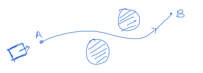
• A robot needs to navigate from point $A$ to point $B$ as quickly as possible without colliding with any obstacles.

  

• Finding minimum energy walking gait for a legged cobot.

• Cloning an acrobatic maneuver on an autonomous helicopter.

Mathematically Speaking

An optimal control problem is an optimization problem where we seek to minimize a cost function subject to system dynamics and other state constraints.

$$\begin{aligned} \text { minimize } & \quad \text{ some objective } \\ \text { subject to } & \quad \text{ system dynamics } \\ & \quad \text { other constraints }\left\{\begin{array}{r} \text { Control bounds } \\ \text { Obstacles } \\ \text { State constraints } \end{array}\right. \end{aligned}$$

Example

To understand this, let's go back to the problem of navigating from point $A$ to point $B$ while spending minimum fuel.

• Cost function - Distance to the point $B$ and the fuel spent.

• System dynamics - Physical Constraints that define robot physics.

• Constraints - Stating the position of the car. Power bounds/control bounds.

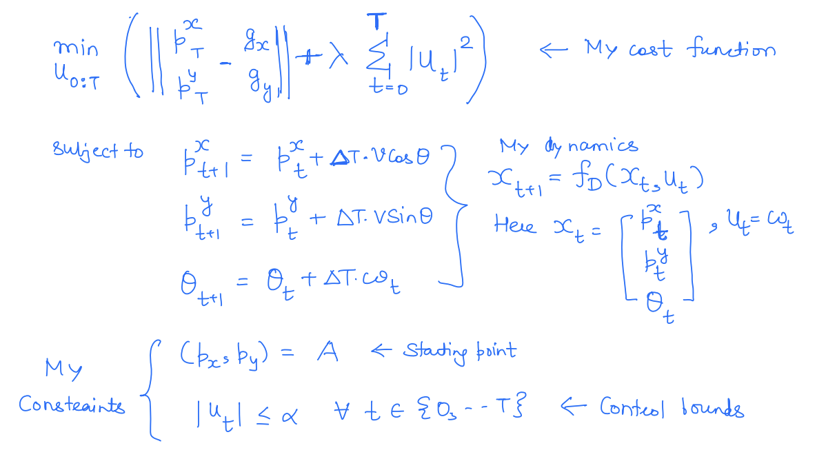
This particular problem above is an instance of a trajectory planning problem in robotics and has several variants where additional constraints (e.g. avoiding obstacles) or alternative cost functions (e.g. minimum time, minimum jerk, etc.) can be used.

Definition

We are now ready to define general optimal control problems.

$$\begin{aligned} \min _{u_{t: T}} \quad & J\left(x_{t}, u_{t: T}, t\right) =\sum_{s=t}^{T-1} L\left(x_{s}, u_{s}\right)+l\left(x_{T}\right) \\ \text { subject to } \quad & x_{s+1} =f_{D}\left(x_{s}, u_{s}\right) \\ & \underline{u} \leq u_{s} \leq \bar{u} \quad \forall s \in\left\{t, t+1, \cdots, T\right\} \end{aligned}$$

• Here, $J\left(x_{t}, u_{t: T}, t\right)$ is the total cost accumulated over the horizon $[t, T]$ starting from the state of $x_{t}$ at time $t$ and applying control $U_{t: T}$.

• $L(\left.x_{s}, u_{s}\right)$ is called the running cost.

• $l\left(x_{T}\right)$ is called the terminal cost (since it only depends on the terminal state). What is the running and terminal cost in the example above?

• There are dynamic constraints. Additionally, there might be control bounds on the system.

• Sometimes optimal control problems are posed in terms of rewards rather than cost, i.e.,

  $$\max _{u_{t: T}} R\left(x_{t}, u_{t: T}, t\right)=\sum \cdots$$

  Now, the control is chosen to maximize the reward. This formulation is particularly popular in Reinforcement Learning. However, the two formulations are equivalent because the negative of the cost function can always be treated as a reward.

note

The same optimal control problem can also be posed in continuous time.

$$\begin{aligned} \min _{u(\cdot)} \quad & J(x(t), u(\cdot), t) =\int_{s=t}^{T} L(x(s), u(s))+l(x(T)) \\ \text { subject to } \quad & \dot{x}(s) =f_{c}(x(s), u(s)) \quad \forall s \in[t, T] \\ & \underline{u} \leq u(s) \leq \bar{u} \end{aligned}$$

The key question here is how to solve this optimal control problem.

Methods to Solve Optimal Control Problems

Given the popularity and ubiquity of optimal control problems in robotics, a variety of methods have been developed to solve such problems:

1. Calculus of Variations $\rightarrow$ Treat it as an optimization problem

2. MPC - Model Predictive Control

3. Dynamic Programming

4. Reinforcement Learning

These different methods make trade-offs in terms of what they need to know about the robotic system and the optimality with which they solve the optimal control problem.

Let's briefly chat about these methods. First of all, recall that the goal of an optimal control problem is to find the optimal control input that minimizes a performance criterion. Mathematically, we are interested in finding the optimal control sequence

$$\begin{aligned} u_{t: T}^{*}=\argmin_{u_{t: T}} & \quad J\left(x_{t}, u_{t: T}, t\right) \\ \text{subject to} & \quad \text{dynamics and control bounds} \end{aligned}$$

Similarly, in continuous time, we are interested in finding the optimal control function:

$$\begin{aligned} u^{*}(\cdot)=\argmin_{u(\cdot)} & \quad J(x(t), u(\cdot), t) \\ \text { subject to } & \quad \dot{x}(s) =f_{c}(x(s), u(s)) \\ & \quad \underline{u} \leq u(s) \leq \bar{u} \end{aligned}$$

Calculus of Variations

The calculus of variations is a field of mathematics concerned with minimizing (or maximizing) functionals, i.e., real-valued functions whose inputs are functions. Our optimal control problem in continuous time falls under this category.

In calculus of variations, the optimal control problem is first converted into an unconstrained optimization problem with the help of Lagrange multipliers. Next, we find the first-order necessary conditions for the optimal solution of this unconstrained optimization problem. These first-order optimality conditions can be used to find a "locally optimal" solution to the optimal control problem.

Mathematically, the problem is a bit involved but I have attempted to provide a snapshot, albeit handwavey, of what it entails.

The unconstrained optimization problem has the following objective (ignoring control bounds for brevity):

$$\begin{aligned} J(x(t), t, u(\cdot), p(\cdot))= & \int_{s=t}^{T} L(x(s), u(s)) ds+l(x(T)) \\ & + \int_{s=t}^{T} p^{T}(f(x(s), u(s))-\dot{x}(s)) ds \end{aligned}$$

Where $p(s) \in \mathbb{R}^{n}$ is the Lagrange multiplier (continuous function in this case since the constraint is continuous). $p(\cdot)$ is also referred to as co-state.

Given the unconstrained optimization problem above, we can assume that around the optimal solution, small variations in $J$ with respect to any variable will be zero. In other words,

$$\frac{\partial J}{\partial x}=0, \frac{\partial J}{\partial b}=0, \frac{\partial J}{\partial u}=0 \text { and so on. }$$

This will result in a bunch of ordinary differential equations that can be solved to obtain $u^{*}(\cdot), x^{*}(\cdot), b^{*}(\cdot)$.

Now, we are ready to discuss the pros and cons of Calculus of Variations.

Pros	Cons
We can use tools from optimization community to solve optimal control problem.	The solution is only locally optimal. It can be globally optimal only if the optimization problem is convex (requires convex objectives and linear dynamics!).
We only need to solve a set of ODEs to find the (locally) optimal solution as opposed to solving a PDE.	Often, we need to solve coupled ODEs which are twice the dimension of the actual system. Can be challenging to do in continuous time for high-dimensional systems.
Can solve the optimal control problem in continuous time.